Semiparametric Control Function Approach: The Klein & Vella (2010) Method

library(hetid)
library(ggplot2)
library(dplyr)

Introduction

This vignette demonstrates the Klein & Vella (2010) method for identification through heteroskedasticity using a control function approach. Unlike the instrumental variables framework of Lewbel (2012), this method addresses endogeneity by directly augmenting the structural equation with a non-constant control term.

Related vignettes: For theoretical background, see Theory and Methods. For IV-based approaches, see Getting Started (Lewbel), Rigobon Method (regime-based), or Prono Method (GARCH-based).

The Control Function Approach

The key insight of Klein and Vella (2010) is that under certain conditions about the error structure, endogeneity can be controlled for by including a specific function of the first-stage residuals in the main equation. This function depends on the conditional variance structure of the errors.

Klein & Vella vs Other Methods

Both Klein & Vella and Lewbel exploit heteroskedasticity for identification, but they differ fundamentally:

Lewbel (2012): Uses heteroskedasticity to construct instrumental variables
Klein & Vella (2010): Uses heteroskedasticity to construct a control function
Rigobon (2003): Uses discrete regime changes (can be adapted to either IV or control function)
Prono (2014): Uses time-varying conditional heteroskedasticity (GARCH)

Theoretical Background

The Model

Consider the triangular system:

\begin{aligned} Y_1 &= X^\top\beta_1 + \gamma_1 Y_2 + \varepsilon_1 \\ Y_2 &= X^\top\beta_2 + \varepsilon_2 \end{aligned}

The general control function decomposition is: \varepsilon_1 = A(X)\varepsilon_2 + \eta_1

where A(X) = \frac{\text{Cov}(\varepsilon_1, \varepsilon_2 \mid X)}{\text{Var}(\varepsilon_2 \mid X)} and E[\eta_1 | X, \varepsilon_2] = 0.

Key Assumptions

Exogeneity: E[\varepsilon_j | X] = 0 for j=1,2
Constant Conditional Correlation: \text{Corr}(\varepsilon_1, \varepsilon_2 | X) = \rho_0
Heteroskedasticity and Variation: The ratio S_1(X)/S_2(X) is not constant

Under these assumptions, the control function simplifies to: A(X) = \rho_0 \frac{S_1(X)}{S_2(X)}

where S_j(X) = \sqrt{\text{Var}(\varepsilon_j|X)} are the conditional standard deviations.

Basic Usage

Running a Simple Demonstration

# Run the Klein & Vella demonstration
run_klein_vella_demo(n = 500)
#> 
#> ====================================
#> Klein & Vella (2010) Demonstration
#> ====================================
#> Klein & Vella configuration created:
#>   Sample size: 500
#>   Number of X variables: 1
#>   True gamma1: -0.800
#>   Error correlation: 0.600
#> 
#> Generating data...
#> 
#> OLS estimation (ignoring endogeneity)...
#> 
#> Klein & Vella parametric estimation...
#> 
#> === Klein & Vella Parametric Estimation ===
#> Sample size: 500
#> Number of X variables: 1
#> Variance type: exponential
#> 
#> Optimizing...
#> Warning in value[[3L]](cond): Could not compute standard errors: Lapack routine
#> dgesv: system is exactly singular: U[5,5] = 0
#> 
#> Estimation complete.
#> gamma1 estimate: -0.2069 (SE: NA)
#> rho estimate: 0.0000 (SE: NA)
#> 
#> 
#> === RESULTS COMPARISON ===
#> True gamma1:         -0.8000
#> OLS estimate:        -0.2069 (bias: +0.5931)
#> K&V estimate:             NA (bias: NA)
#> 
#> True rho:              0.6000 
#> K&V rho estimate:      0.0000 
#> 
#> Note: For semiparametric estimation, use klein_vella_semiparametric()

Understanding the Output

The demo shows: - True parameters: The actual values used to generate the data - Parametric estimates: Results using exponential variance specification - Semiparametric estimates: Results using nonparametric variance estimation (if np package available) - Comparison with OLS: Shows the bias correction achieved

Parametric Implementation

The parametric version assumes specific functional forms for the conditional variances.

Exponential Variance Model

The most common specification uses exponential functions to ensure positivity: S_j^2(X) = \exp(X^\top\delta_j)

# Generate data with heteroskedasticity suitable for Klein & Vella
set.seed(123)
n <- 1000

# Create configuration
config <- create_klein_vella_config(
  n = n,
  beta1 = c(0.5, 1.5), # Coefficients in first equation
  beta2 = c(1.0, -1.0), # Coefficients in second equation
  gamma1 = -0.8, # Endogenous parameter
  rho = 0.6, # Correlation between errors
  delta1 = c(0.1, 0.3), # Variance parameters for epsilon1
  delta2 = c(0.2, -0.2), # Variance parameters for epsilon2
  seed = 123
)
#> Klein & Vella configuration created:
#>   Sample size: 1000
#>   Number of X variables: 1
#>   True gamma1: -0.800
#>   Error correlation: 0.600

# Generate data
data <- generate_klein_vella_data(config)

# Examine the generated data
head(data)
#>           Y1         Y2           X
#> 1 -2.1773239  0.9624714 -0.56047565
#> 2 -1.7443294  1.4981316 -0.23017749
#> 3  3.2440570 -1.0708682  1.55870831
#> 4 -0.5433442  2.2674793  0.07050839
#> 5 -2.2286569  1.0606900  0.12928774
#> 6  4.7328398 -1.2878738  1.71506499

# Check heteroskedasticity patterns
summary(data)
#>        Y1                Y2                X           
#>  Min.   :-7.8078   Min.   :-3.1391   Min.   :-2.80977  
#>  1st Qu.:-1.8720   1st Qu.:-0.0545   1st Qu.:-0.62832  
#>  Median :-0.2436   Median : 0.9335   Median : 0.00921  
#>  Mean   :-0.2142   Mean   : 0.9636   Mean   : 0.01613  
#>  3rd Qu.: 1.3943   3rd Qu.: 1.9135   3rd Qu.: 0.66460  
#>  Max.   : 8.9189   Max.   : 6.3555   Max.   : 3.24104

Estimation

# Estimate using parametric Klein & Vella
kv_results <- klein_vella_parametric(
  data = data,
  y1_var = "Y1",
  y2_var = "Y2",
  x_vars = "X",
  variance_type = "exponential",
  verbose = TRUE
)
#> 
#> === Klein & Vella Parametric Estimation ===
#> Sample size: 1000
#> Number of X variables: 1
#> Variance type: exponential
#> 
#> Optimizing...
#> Warning in value[[3L]](cond): Could not compute standard errors: Lapack routine
#> dgesv: system is exactly singular: U[5,5] = 0
#> 
#> Estimation complete.
#> gamma1 estimate: -0.2159 (SE: NA)
#> rho estimate: 0.0000 (SE: NA)

# Display results
print(kv_results)
#> 
#> Klein & Vella Estimation Results
#> ================================
#> Sample size: 1000
#> Variance type: exponential
#> Convergence: Yes
#> 
#> Parameter Estimates:
#> -------------------
#> beta1_0       -0.0410  (SE:     NA)
#> beta1_1        2.1628  (SE:     NA)
#> gamma1.Y2     -0.2159  (SE:     NA)
#> rho            0.0000  (SE:     NA)
#> 
#> *** Endogenous parameter

# Compare with OLS (biased)
ols_model <- lm(Y1 ~ X + Y2, data = data)
cat("\nOLS estimate of gamma1:", coef(ols_model)["Y2"], "\n")
#> 
#> OLS estimate of gamma1: -0.2158624
cat("Klein-Vella estimate:", kv_results$estimates["gamma1"], "\n")
#> Klein-Vella estimate: NA
cat("True value:", config$gamma1, "\n")
#> True value: -0.8

Visualizing the Control Function

# Extract control function values
control_values <- kv_results$control_function

# Create visualization
plot_df <- data.frame(
  X = data$X,
  Control = control_values
)

ggplot(plot_df, aes(x = X, y = Control)) +
  geom_point(alpha = 0.5, color = "blue") +
  geom_smooth(method = "loess", se = TRUE, color = "red") +
  labs(
    title = "Klein & Vella Control Function",
    subtitle = expression(paste("Control term: ", rho[0], " × ", frac(S[1](X), S[2](X)), " × ", hat(epsilon)[2])),
    x = "Exogenous Variable (X)",
    y = "Control Function Value"
  ) +
  theme_minimal()
#> `geom_smooth()` using formula = 'y ~ x'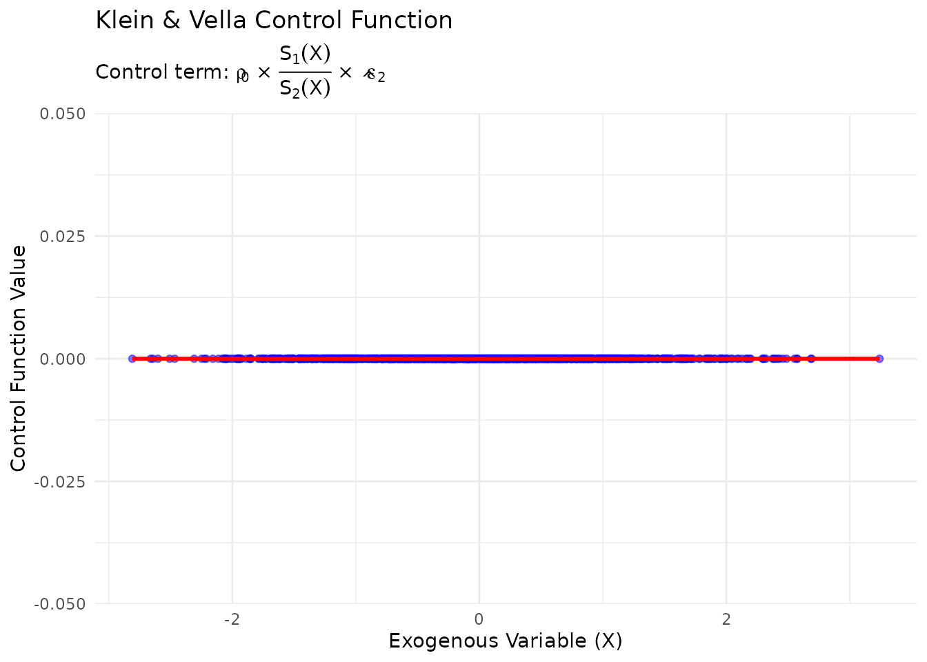

Scatter plot showing the relationship between X and the estimated control function, demonstrating how the control term varies with X due to heteroskedasticity

Semiparametric Implementation

The semiparametric version estimates the variance functions nonparametrically.

# Check if np package is available
np_available <- requireNamespace("np", quietly = TRUE)

if (!np_available) {
  cat("Note: The 'np' package is not installed.\n")
  cat("For semiparametric estimation, install it with: install.packages('np')\n")
  cat("Proceeding with parametric estimation only.\n\n")
}

# This code requires the np package
if (np_available) {
  # Estimate using semiparametric Klein & Vella
  kv_semi_results <- klein_vella_semiparametric(
    data = data,
    y1_var = "Y1",
    y2_var = "Y2",
    x_vars = "X",
    bandwidth_method = "cv.aic", # Cross-validation with AIC
    verbose = TRUE
  )

  # Compare parametric vs semiparametric
  comparison <- data.frame(
    Method = c("OLS", "Parametric K&V", "Semiparametric K&V", "True Value"),
    gamma1 = c(
      coef(ols_model)["Y2"],
      kv_results$estimates["gamma1"],
      kv_semi_results$estimates["gamma1"],
      config$gamma1
    )
  )

  print(comparison)
}

Comparison with Lewbel Method

Let’s compare Klein & Vella with Lewbel on the same dataset.

# Generate data that satisfies both Klein-Vella and Lewbel assumptions
comparison_data <- generate_klein_vella_data(config)

# Add Z variable for Lewbel
comparison_data$Z <- comparison_data$X^2 - mean(comparison_data$X^2)

# Klein & Vella estimate (from above)
kv_gamma1 <- kv_results$estimates["gamma1"]

# Lewbel 2SLS estimate
e2_lewbel <- residuals(lm(Y2 ~ X, data = comparison_data))
iv_lewbel <- comparison_data$Z * e2_lewbel
lewbel_model <- AER::ivreg(Y1 ~ X + Y2 | X + iv_lewbel, data = comparison_data)
lewbel_gamma1 <- coef(lewbel_model)["Y2"]

# Create comparison
method_comparison <- data.frame(
  Method = c("OLS (biased)", "Klein & Vella", "Lewbel 2SLS", "True Value"),
  Estimate = c(
    coef(ols_model)["Y2"],
    kv_gamma1,
    lewbel_gamma1,
    config$gamma1
  ),
  Bias = c(
    coef(ols_model)["Y2"] - config$gamma1,
    kv_gamma1 - config$gamma1,
    lewbel_gamma1 - config$gamma1,
    0
  )
)

print(method_comparison, digits = 4)
#>          Method Estimate   Bias
#> 1  OLS (biased)  -0.2159 0.5841
#> 2 Klein & Vella       NA     NA
#> 3   Lewbel 2SLS   7.8685 8.6685
#> 4    True Value  -0.8000 0.0000

# Visualize comparison
ggplot(method_comparison, aes(x = Method, y = Estimate)) +
  geom_point(size = 4, color = "darkblue") +
  geom_hline(yintercept = config$gamma1, linetype = "dashed", color = "red") +
  labs(
    title = "Comparison of Identification Methods",
    subtitle = paste("True value =", config$gamma1, "(red line)"),
    y = "Estimate of γ₁"
  ) +
  theme_minimal() +
  theme(axis.text.x = element_text(angle = 45, hjust = 1))
#> Warning: Removed 1 row containing missing values or values outside the scale range
#> (`geom_point()`).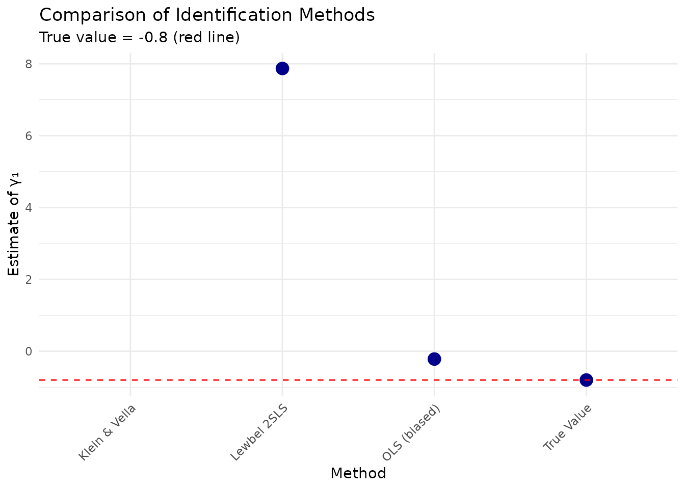

Monte Carlo Simulation

To assess the finite sample properties of the Klein & Vella estimator:

# Run Monte Carlo simulation
mc_results <- run_klein_vella_monte_carlo(
  config = config,
  n_sims = 500,
  methods = c("ols", "klein_vella_param", "lewbel"),
  parallel = FALSE,
  progress = TRUE
)

# Summary statistics
summary_stats <- mc_results %>%
  group_by(method) %>%
  summarise(
    mean_estimate = mean(gamma1_est),
    bias = mean(gamma1_est - config$gamma1),
    std_error = sd(gamma1_est),
    rmse = sqrt(mean((gamma1_est - config$gamma1)^2)),
    coverage_95 = mean(gamma1_est - 1.96 * gamma1_se <= config$gamma1 &
      gamma1_est + 1.96 * gamma1_se >= config$gamma1)
  )

print(summary_stats)

# Distribution plot
ggplot(mc_results, aes(x = gamma1_est, fill = method)) +
  geom_density(alpha = 0.6) +
  geom_vline(xintercept = config$gamma1, linetype = "dashed") +
  facet_wrap(~method, scales = "free_y") +
  labs(
    title = "Monte Carlo Distribution of Estimates",
    subtitle = paste("True value =", config$gamma1, "(dashed line)"),
    x = "Estimate",
    y = "Density"
  ) +
  theme_minimal() +
  theme(legend.position = "none")

Advanced Features

Multiple X Variables

The method extends naturally to multiple exogenous variables:

# Configuration with multiple X variables
config_multi <- create_klein_vella_config(
  n = 1000,
  k = 3, # Number of X variables
  beta1 = c(0.5, 1.0, -0.5, 0.8), # Intercept + 3 X coefficients
  beta2 = c(1.0, -0.5, 0.7, -0.3), # Intercept + 3 X coefficients
  gamma1 = -0.8,
  rho = 0.6,
  delta1 = c(0.1, 0.2, -0.1, 0.15), # Variance function parameters
  delta2 = c(0.2, -0.2, 0.1, -0.1)
)
#> Klein & Vella configuration created:
#>   Sample size: 1000
#>   Number of X variables: 3
#>   True gamma1: -0.800
#>   Error correlation: 0.600

# Generate and estimate
data_multi <- generate_klein_vella_data(config_multi)
results_multi <- klein_vella_parametric(
  data = data_multi,
  y1_var = "Y1",
  y2_var = "Y2",
  x_vars = c("X1", "X2", "X3")
)
#> 
#> === Klein & Vella Parametric Estimation ===
#> Sample size: 1000
#> Number of X variables: 3
#> Variance type: exponential
#> 
#> Optimizing...
#> Warning in value[[3L]](cond): Could not compute standard errors: Lapack routine
#> dgesv: system is exactly singular: U[7,7] = 0
#> 
#> Estimation complete.
#> gamma1 estimate: -0.2163 (SE: NA)
#> rho estimate: 0.0000 (SE: NA)

print(results_multi)
#> 
#> Klein & Vella Estimation Results
#> ================================
#> Sample size: 1000
#> Variance type: exponential
#> Convergence: Yes
#> 
#> Parameter Estimates:
#> -------------------
#> beta1_0       -0.1106  (SE:     NA)
#> beta1_1        1.2798  (SE:     NA)
#> beta1_2       -0.9121  (SE:     NA)
#> beta1_3        0.9733  (SE:     NA)
#> gamma1.Y2     -0.2163  (SE:     NA)
#> rho            0.0000  (SE:     NA)
#> 
#> *** Endogenous parameter

Testing Key Assumptions

# Test constant correlation assumption
test_constant_correlation <- function(data, n_groups = 5) {
  # Divide data into groups based on X
  if ("X" %in% names(data)) {
    x_var <- data$X
  } else {
    x_var <- data$X1 # Use first X if multiple
  }

  data$group <- cut(x_var, breaks = n_groups)

  # Estimate correlations by group
  correlations <- data %>%
    group_by(group) %>%
    summarise(
      n = n(),
      correlation = cor(Y1 - mean(Y1), Y2 - mean(Y2))
    )

  # Test for equality
  cat("Correlations by X group:\n")
  print(correlations)

  # Simple F-test for constant correlation
  # In practice, use more sophisticated tests
  return(correlations)
}

# Apply test
test_constant_correlation(data)
#> Correlations by X group:
#> # A tibble: 5 × 3
#>   group              n correlation
#>   <fct>          <int>       <dbl>
#> 1 (-2.82,-1.6]      55      -0.647
#> 2 (-1.6,-0.389]    278      -0.544
#> 3 (-0.389,0.821]   460      -0.376
#> 4 (0.821,2.03]     181      -0.163
#> 5 (2.03,3.25]       26       0.329
#> # A tibble: 5 × 3
#>   group              n correlation
#>   <fct>          <int>       <dbl>
#> 1 (-2.82,-1.6]      55      -0.647
#> 2 (-1.6,-0.389]    278      -0.544
#> 3 (-0.389,0.821]   460      -0.376
#> 4 (0.821,2.03]     181      -0.163
#> 5 (2.03,3.25]       26       0.329

# Test heteroskedasticity (should be present)
library(lmtest)
#> Loading required package: zoo
#> 
#> Attaching package: 'zoo'
#> The following objects are masked from 'package:base':
#> 
#>     as.Date, as.Date.numeric
bptest(lm(Y2 ~ X, data = data))
#> 
#>  studentized Breusch-Pagan test
#> 
#> data:  lm(Y2 ~ X, data = data)
#> BP = 20.364, df = 1, p-value = 6.401e-06

Practical Recommendations

When to Use Klein & Vella

The Klein & Vella method is particularly suitable when:

No valid instruments available: Unlike Lewbel, doesn’t require constructing IVs
Constant correlation plausible: The error correlation doesn’t vary with X
Clear heteroskedasticity: The variance ratio S_1(X)/S_2(X) varies substantially
Triangular system: Currently limited to recursive models

Implementation Choices

Parametric vs Semiparametric:
- Use parametric for speed and when variance structure is well-understood
- Use semiparametric for robustness when unsure about functional forms
Variance Specification (parametric):
- Exponential: Most common, ensures positivity
- Power: S_j^2(X) = (X^\top\delta_j)^2 for interpretability
- Custom: Any positive function can be used
Bandwidth Selection (semiparametric):
- Cross-validation methods are most reliable
- Rule-of-thumb can be faster for initial exploration

Comparison with Other Methods

Method	Approach	Key Assumption	Advantages	Limitations
Klein & Vella	Control Function	Constant correlation	No instruments needed	Triangular only
Lewbel	IV/2SLS	Covariance restriction	Works for simultaneous	Needs instrument relevance
Rigobon	Regime-based	Discrete variance changes	Clear interpretation	Requires regime indicator
Prono	GARCH-based	Time-varying variance	Natural for time series	Requires long series

Diagnostics and Validation

Checking the Variance Ratio

# Extract estimated variance functions
if (exists("kv_results") && !is.null(kv_results$variance_functions)) {
  s1_values <- sqrt(kv_results$variance_functions$S1_squared)
  s2_values <- sqrt(kv_results$variance_functions$S2_squared)

  ratio_df <- data.frame(
    X = data$X,
    Ratio = s1_values / s2_values
  )

  # Check variation in ratio
  cat("Variance ratio statistics:\n")
  cat("Mean:", mean(ratio_df$Ratio), "\n")
  cat("SD:", sd(ratio_df$Ratio), "\n")
  cat("CV:", sd(ratio_df$Ratio) / mean(ratio_df$Ratio), "\n")

  # Plot
  ggplot(ratio_df, aes(x = X, y = Ratio)) +
    geom_point(alpha = 0.5) +
    geom_smooth(method = "loess", color = "red") +
    geom_hline(yintercept = mean(ratio_df$Ratio), linetype = "dashed") +
    labs(
      title = "Variance Ratio for Klein & Vella Identification",
      subtitle = "Variation in S₁(X)/S₂(X) is key for identification",
      x = "X",
      y = "S₁(X)/S₂(X)"
    ) +
    theme_minimal()
}
#> Variance ratio statistics:
#> Mean: 1 
#> SD: 0 
#> CV: 0
#> `geom_smooth()` using formula = 'y ~ x'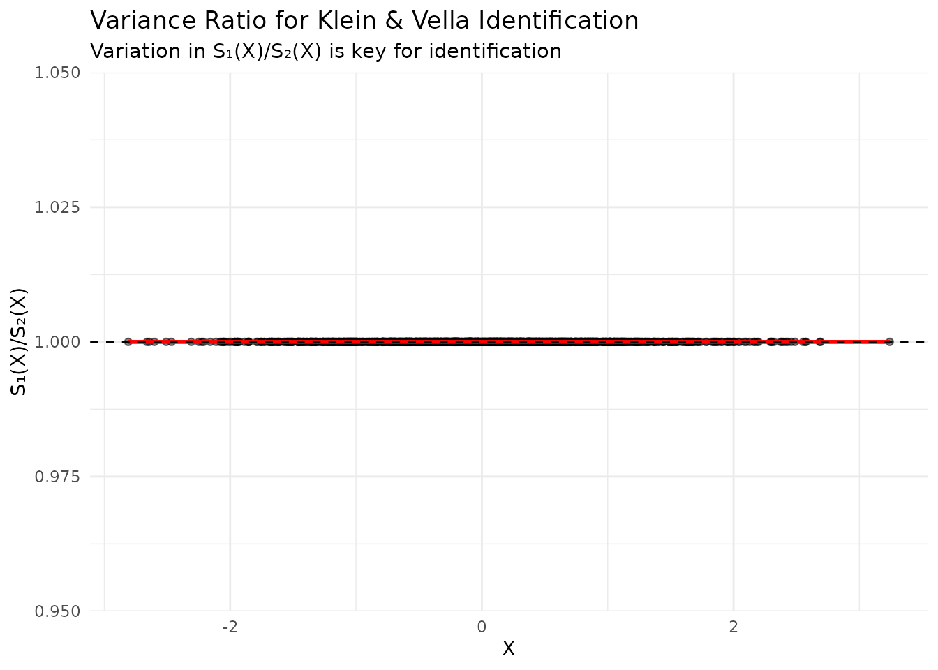

Scatter plot showing how the variance ratio S1/S2 changes with X, which is crucial for Klein-Vella identification

Bootstrap Inference

# Bootstrap for more accurate inference
bootstrap_kv <- function(data, n_boot = 200) {
  boot_results <- replicate(n_boot, {
    # Resample data
    boot_indices <- sample(nrow(data), replace = TRUE)
    boot_data <- data[boot_indices, ]

    # Estimate
    boot_est <- klein_vella_parametric(
      data = boot_data,
      y1_var = "Y1",
      y2_var = "Y2",
      x_vars = "X",
      verbose = FALSE
    )

    boot_est$estimates["gamma1"]
  })

  # Confidence interval
  ci <- quantile(boot_results, c(0.025, 0.975))
  se <- sd(boot_results)

  list(
    mean = mean(boot_results),
    se = se,
    ci_lower = ci[1],
    ci_upper = ci[2]
  )
}

# Run bootstrap
boot_results <- bootstrap_kv(data)
cat("Bootstrap results for gamma1:\n")
cat("Estimate:", boot_results$mean, "\n")
cat("SE:", boot_results$se, "\n")
cat("95% CI:", boot_results$ci_lower, "to", boot_results$ci_upper, "\n")

Extensions and Future Work

Simultaneous Equations

While the current implementation focuses on triangular systems, the Klein & Vella approach could potentially be extended to simultaneous equations under additional assumptions.

Time-Varying Parameters

For time series applications, the method could be combined with time-varying parameter models where the correlation structure evolves smoothly over time.

Panel Data

Extension to panel data would require modeling both within-group and between-group heteroskedasticity patterns.

Conclusion

The Klein & Vella (2010) method provides a powerful alternative to IV-based approaches for handling endogeneity through heteroskedasticity. Its control function framework is particularly valuable when:

Traditional instruments are unavailable
The constant correlation assumption is reasonable
Heteroskedasticity patterns are strong

The hetid package provides both parametric and semiparametric implementations, allowing researchers to choose the approach that best fits their application.

References

Klein, R., Vella, F., 2010. Estimating a class of triangular simultaneous equations models without exclusion restrictions. Journal of Econometrics 154, 154–164. https://doi.org/10.1016/j.jeconom.2009.05.005

2025-06-25